NSFsim: Validation and Verification of Synthetic Magnetic Diagnostics
In our previous post about NSFsim, we explained the process of digital replica validation to ensure precise simulations of tokamaks. Since NSFsim is the cornerstone of all our other products, its validation using experimental data is an essential step to ensure the feasibility and applicability of NSFsim.
For example, our recent work has focused on training plasma shape and position control models using reinforcement learning (RL). Realistic and precise simulation of magnetic probes and flux loops is essential for creating a proper RL training environment.
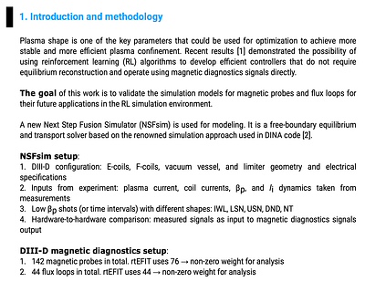
NSFsim is a free-boundary equilibrium and transport solver. To solve the Grad-Shafranov equation for a specific tokamak, the electric representation of this tokamak is required. This involves specifying the poloidal field coils, vacuum vessel, and limiter geometry, along with their electrical characteristics. Furthermore, magnetic probe and loop signals are calculated by considering the mutual magnetic fields arising from plasma currents, and both active and passive elements.
In this post, we examine the recent results of validating NSFsim and the digital replica of the DIII-D tokamak against DIII-D’s experimental data and GSevolve, DIII-D’s own simulator.
The Approach
The simulator is used in reproduction mode and utilizes the dynamics of measured plasma and PF-coil currents as input parameters, along with kinetic profiles from EFIT. Five configurations are considered: lower single null (LSN), upper single null (USN), double null (DN), inner wall limited (IWL), and negative triangularity (NT). Results obtained via NSFsim are compared with experimental data and GSevolve simulations.
This approach enables us to perform hardware-to-hardware comparisons, ensuring that equilibrium and synthetic magnetic signals closely reproduce experimental data.
The Data

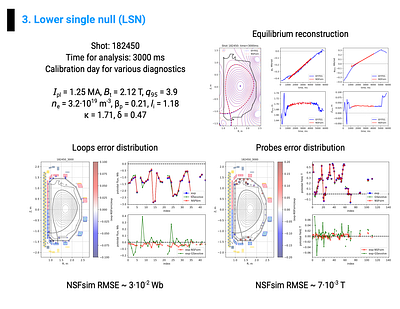


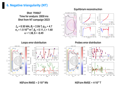
The top right plot shows how well the equilibrium is reproduced. It is represented by the 2D distribution of normalized poloidal flux 𝜓ₙ(R,Z), the absolute values of poloidal flux at the plasma center and boundary, and the coordinates of the magnetic axis. The bottom left (for loops) and right (for probes) plots show the accuracy of the simulation. The locations of sensors are shown on the poloidal cross-section by circles of different colors and sizes. The color indicates the relative error according to the color bar, and the size represents the value of the absolute error, so small white circles indicate an excellent match.
The Results
A perfect match is obtained for loop signals.
Probes are more difficult to model since they are more sensitive to local field disturbances, such as induced currents and 3D coils that are not included in 2D simulations. Good agreement is observed for most of the probes, but there are noticeable discrepancies in the divertor regions and near the F6B and F7B coils. A more detailed model of the vacuum vessel and passive elements is required to improve accuracy, but it leads to slower calculations, which is not tolerable in machine learning tasks.
Overall, NSFsim’s RMSE in this validation project demonstrates the consistently high quality of simulations provided by NSFsim and the advantages of its configurable and modular approach.
In future posts, we will show more examples of precise simulations using NSFsim and explain how you can use it directly in your web browser, without any additional software or hardware.
Stay tuned!