NSFsim: What's the novelty in our tokamak simulator
A summary of recent developments and next steps in the NSFsim simulation environment
A tokamak simulator is useful only if it balances physics fidelity with practical modeling workflows. It must solve well-defined plasma physics problems for scenario design, reconstruction, and control studies while remaining usable for coupling to external codes and for comparison with experiments. In recent development cycles, the Next Step Fusion Simulator (NSFsim) has been extended in this direction: the core numerical workflow has been improved, several modules have become more physically transparent, and new physics components are being prepared for integration.
This post summarizes the current state of NSFsim, explains what has changed, and outlines the next steps on the roadmap. The focus is not only on individual features but also on how the modules integrate to form a broader simulation environment for tokamak design, operation, and control-oriented modeling.
What is NSFsim?
NSFsim is an advanced 2D Grad–Shafranov solver coupled with a 1D radial kinetic component. It supports a broad range of tokamak modeling tasks, including direct equilibrium calculations, discharge-scenario modeling, inverse equilibrium design, equilibrium reconstruction, disruption simulations, and self-consistent coupling to external physics codes. The simulator is IMAS-compatible and available for academic use via the cloud-based Fusion Twin Platform API. Interfaces are provided for Python, MATLAB, and C++.
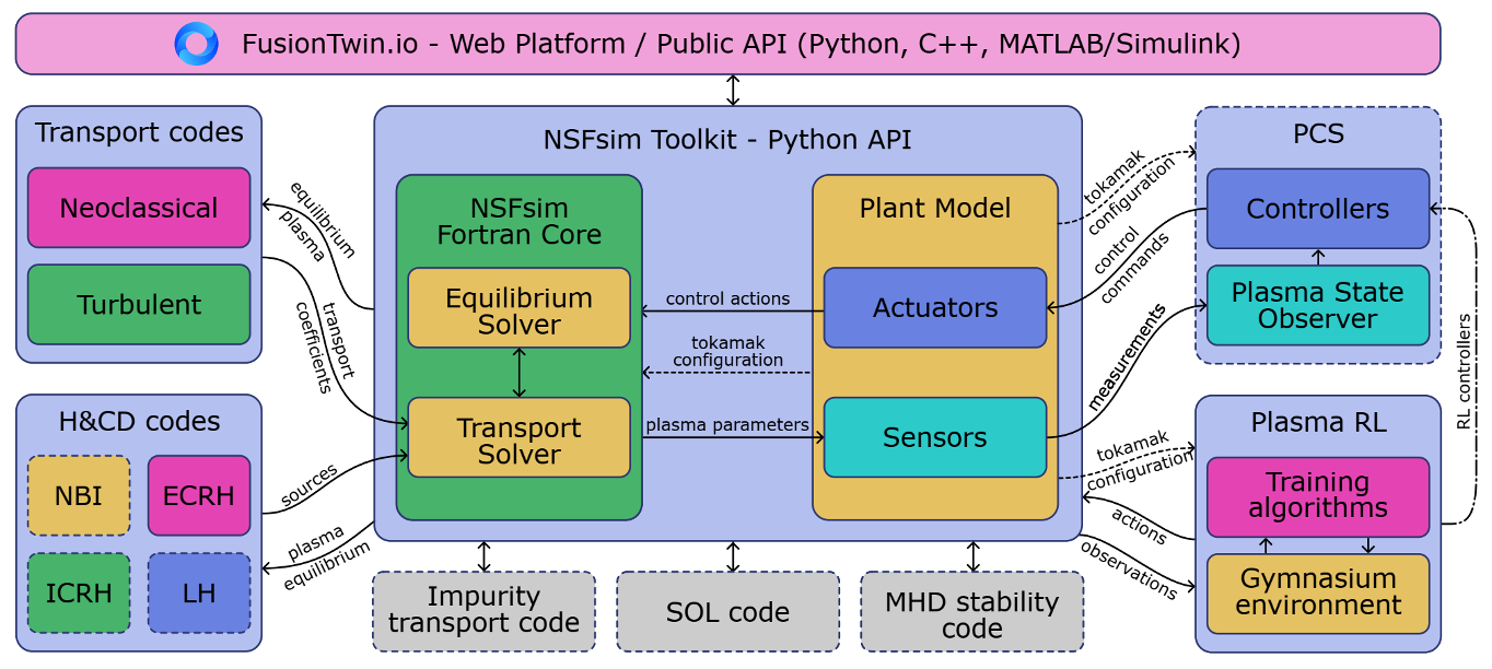
The general architecture reflects NSFsim's core design principle: the equilibrium solver should not be an isolated numerical component. It should serve as the central physics layer, exchanging information with transport models, heating and current-drive codes, plant models, controllers, reconstruction tools, and machine-learning environments.
Forward calculation: the main simulation mode
The forward, or direct, calculation is NSFsim's primary operating mode. Given coil currents/voltages and kinetic plasma parameters, the simulator computes the plasma equilibrium, poloidal-flux evolution, and radial profiles of temperature and density. This module has received the most updates because it sits at the center of most workflows: device validation, scenario optimization, external-code coupling, and controller training.
Shared-memory coupling to external codes
A major improvement is the shared-memory coupling mechanism. It allows selected variables to be provided by external codes, evolved internally by NSFsim, or updated through a combined workflow. The purpose is to avoid unnecessary disk I/O and to make coupled simulations fast enough for iterative studies.
This coupling approach has already been implemented with two external codes: TRAVIS and ASCOT5.
TRAVIS for ECRH and ECCD modeling
TRAVIS is a multi-beam, multi-pass ray-tracing code for electron-cyclotron heating and current drive, developed at IPP Max Planck [1]. In the coupled workflow, NSFsim provides the plasma equilibrium, and TRAVIS returns the heating power and driven current profiles. The NSFsim–TRAVIS combination also serves as the simulation core of our machine-learning-based plasma control pipeline.
ASCOT5 for NBI and fast-particle modeling
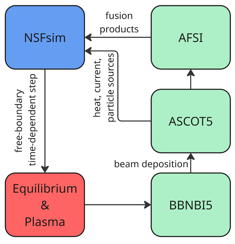
ASCOT5 is an orbit-following Fokker–Planck solver with OpenMP and GPU parallelization [2]. In the implemented workflow, NSFsim provides the equilibrium and plasma background. BBNBI5 computes neutral-beam deposition and shine-through, ASCOT5 calculates fast-ion slowing down, and AFSI evaluates fusion-product sources. Data are exchanged between time steps via shared memory.
This work was carried out in collaboration with VTT, and the coupling scheme is planned for release in the open-source ASCOT5 repository.
EPED-like pedestal workflow
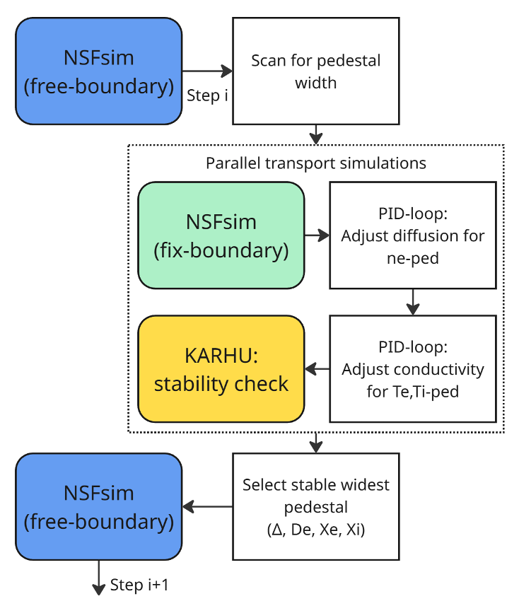
NSFsim now includes an EPED-like workflow for self-consistent pedestal determination. The workflow uses the KARHU v2.0 neural network, trained on HELENA and MISHKA calculations from the JET and DIII-D datasets, to perform MHD stability checks within the NSFsim loop.
For a prescribed pedestal density, the algorithm scans the pedestal width while PID loops adjust particle diffusion and heat conductivity. KARHU rejects unstable configurations, and the widest stable pedestal is selected for the next free-boundary time step. This provides a practical route to pedestal estimation without decoupling equilibrium evolution from stability assessment.
Virtual vertical and horizontal stabilization
A virtual-field stabilization mechanism has been added to NSFsim to control the magnetic-axis position. It has two related uses.
The first is physics-oriented: the plasma column position can be evolved consistently while an ADRC controller minimizes the position error. The second is control-oriented: the same mechanism can serve as a training environment for machine-learning controllers. In that case, the algorithm learns to minimize the virtual fields required to reach a target plasma position without explicit labels for the "correct" coil-current commands.
This is useful for developing control strategies before committing to a particular actuator model or controller architecture.
Switching between free-boundary and fixed-boundary calculations
NSFsim now supports switching between free-boundary and fixed-boundary equilibrium modes. A new fixed-boundary forward solver is in final testing. Its architecture is designed to enable rapid replacement of transport modules, making it easier to compare transport models, test simplified physics assumptions, and couple NSFsim to external transport codes without having to run a full free-boundary calculation at every step.
This capability is especially important for development workflows that require rapid iteration while keeping the calculation aligned with the same equilibrium and profile conventions used in the full model.
Extended source terms and boundary conditions
The forward module has also been extended to provide more flexible handling of sources and boundary conditions. It now supports switching between Dirichlet and Robin boundary conditions, controlling one-dimensional radial-grid uniformity, separate ion and electron heating channels, externally supplied power-deposition profiles, current-drive profiles specified either externally or via internal scaling laws, and arbitrary particle-source profiles.
These additions make the forward solver easier to use in integrated modeling studies, where the plasma state is often determined by several heating, fueling, and current-drive systems rather than by a single prescribed source term.
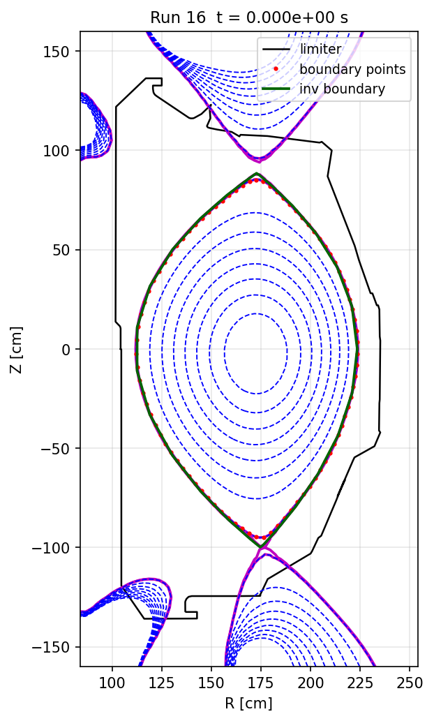
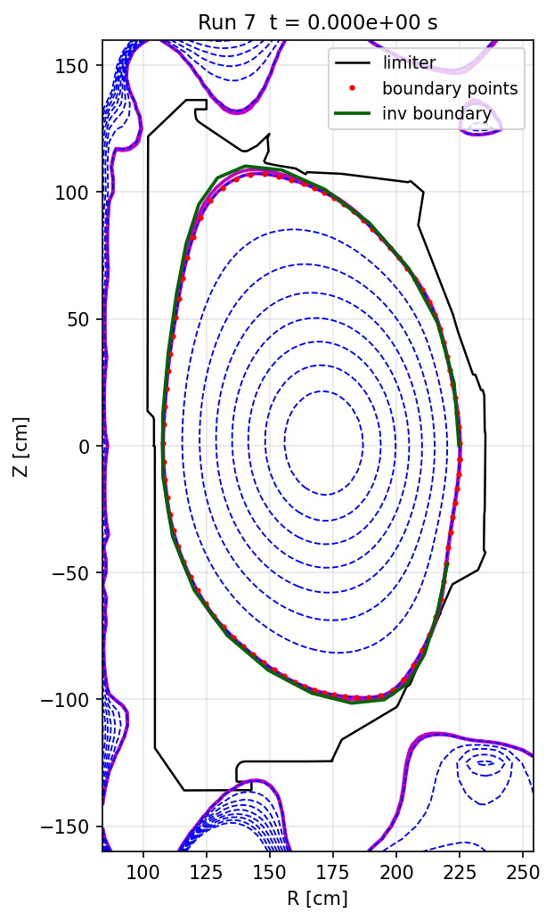
Inverse solver: from numerical surrogates to physical inputs
The inverse solver addresses the complement of the forward problem: given a desired static plasma state, find the coil currents that realize it.
The main update is the transition to physical input parameters. Earlier versions required initialization with quantities such as derivatives of pressure and poloidal current functions. These quantities are mathematically natural for Grad–Shafranov calculations, but they are not convenient inputs for design studies because they are not the parameters users typically want to prescribe.
The new workflow accepts physical quantities directly: desired current density, electron and ion temperature profiles, and density profiles. NSFsim then constructs a consistent initial state by solving for the desired plasma configuration under the given external currents, without requiring the user to specify intermediate numerical surrogates.
Another important improvement is the stabilized transfer of inverse solver results into the forward calculation as initial conditions. This closes the inverse-to-direct loop and reduces dependence on equilibrium-reconstruction codes such as EFIT or on experimental equilibrium data when setting up synthetic or design-oriented simulations.
Scenario builder: evolving a discharge, not only a state
Static equilibrium is often only the starting point. For many applications, the more important question is how coil currents and voltages must evolve so that the plasma follows a prescribed trajectory for shape and parameters. This is the role of the scenario builder.
The scenario builder module can be viewed as an evolutionary inverse solver. It calculates the time evolution of actuator commands needed to reproduce or design a discharge. This makes it relevant for pulse planning, ramp-up studies, current-profile evolution, and the preparation of simulations that must remain close to experimentally feasible operating conditions.
Flexible coil current management
Each coil can now be assigned independent behavior based on the discharge phase or trigger condition. For example, a coil current may evolve freely until a condition is met, then freeze; it may ramp down to zero within a specified interval; or it may follow a prescribed waveform during a selected phase of the discharge.
This level of control makes it easier to reproduce real experimental protocols and to design scenarios with a controlled number of active degrees of freedom. It also helps build simulations that are more likely to be reproducible on actual tokamaks, including cases where full-shape or vertical-stabilization controllers are not yet implemented.
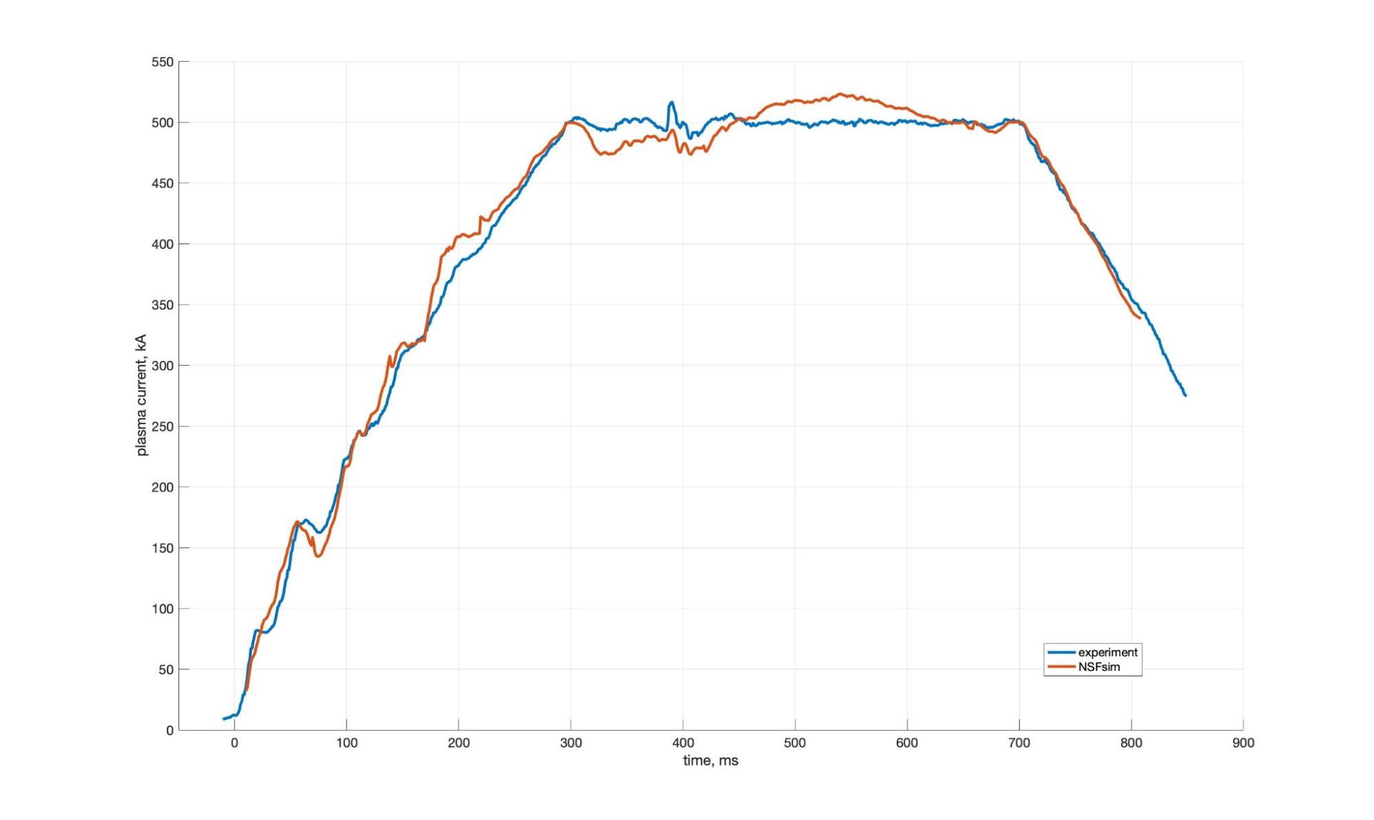
Reproducing discharges from limited experimental data
A workflow has been developed to initialize scenarios using only a limited set of experimental inputs: coil currents, plasma current, and an approximate plasma shape. Tests on several devices show agreement with the experimental state within approximately 5–10%, which is sufficient as a starting point for more detailed modeling.
This is particularly useful during early ramp-up, when magnetic reconstruction can be less reliable, and equilibrium data may be incomplete or difficult to interpret.
Disruption module: connection to 3D structure currents
The disruption module, including calculations for major disruptions and vertical displacement events, has been discussed in detail in earlier posts:
Part 1: NSFSim Perspective on Disruptions in Tokamaks — Part I: Physics Basis
Part 2: NSFsim Perspective on Disruptions in Tokamaks — Part II: Simulations for DTT
Here, the main update is its planned integration with calculations of 3D currents in conducting tokamak structures.
This integration is important because disruption loads are not determined by plasma evolution alone. Eddy and halo currents, passive structures, and plasma motion interact dynamically. A disruption model that can exchange information with a three-dimensional conducting-structure module can therefore provide a more complete basis for structural-load estimation.
The "What comes next" section describes this planned direction in more detail.
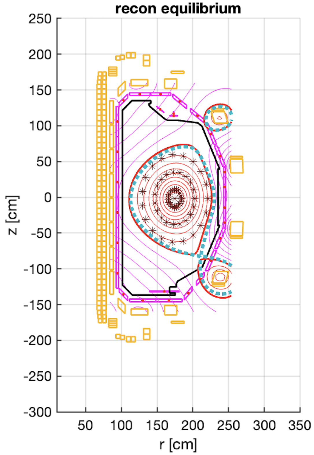
Equilibrium reconstruction: EdFIT
The equilibrium reconstruction module, internally known as EdFIT, reconstructs the magnetic plasma state from diagnostic signals, including plasma current, coil currents, flux loops, and magnetic-probe measurements.
The module is intended to provide reconstruction capabilities consistent with the NSFsim modeling environment while supporting workflows familiar from experimental equilibrium analysis.
Fixed and floating filaments
Two reconstruction modes are now supported. In fixed-filament mode, the current-distribution structure is specified in advance. This is useful when the reconstruction problem must remain constrained or computationally simple.
In floating-filament mode, both the positions and strengths of the current filaments are optimized during reconstruction. This improves flexibility and can increase accuracy in complex plasma configurations where a fixed-current representation is too restrictive.
Configurable iteration triggers
The convergence criteria for a single time step can now be adjusted via external triggers. This allows the user to choose the appropriate balance between speed and accuracy for a given task. A fast reconstruction may be sufficient for control-oriented workflows, while a more converged solution may be needed for analysis or benchmarking.
External poloidal-beta evolution
The module can also accept externally prescribed poloidal-beta evolution. This improves the reproduction of experimental discharge conditions when EdFIT is used as a data source for the forward solver.
Diagnostic signal weighting
An error-weighting mechanism for magnetic diagnostics has been implemented. Unreliable or noisy sensors can be down-weighted or excluded from the reconstruction. This mirrors standard experimental practice, in which problematic magnetic loops are often disabled or assigned a lower weight during EFIT analysis.
What comes next
The current updates improve NSFsim's internal consistency and usability. The next development steps extend the simulator to areas important for reactor-relevant modeling: 3D currents in conducting structures, aneutronic fusion reactions, and scrape-off-layer modeling.
3D electromagnetic currents in conducting structures
We are developing a module to calculate the evolution of eddy and halo currents in passive tokamak structures. The initial formulation uses a thin-wall conducting-shell approach, with the longer-term goal of extending the method to a fully 3D treatment.
A key distinction from some existing thin-wall tools is the physical scope. Many formulations focus on inductive currents that satisfy current continuity on a closed conducting surface. This is a clean and useful problem, and it can naturally be expressed in terms of a scalar current potential.
The NSFsim development path also includes source-driven currents, especially halo currents that enter conducting structures from the plasma and close through them. This capability is necessary for more complete structural-load calculations during vertical displacement events.
Two-way coupling is also under development. In this workflow, 3D structure currents modify the 2D plasma equilibrium, and the updated equilibrium is then used to recalculate the 3D current distribution at the next time step. The goal is a self-consistent plasma–structure interaction model suitable for disruption and VDE studies.
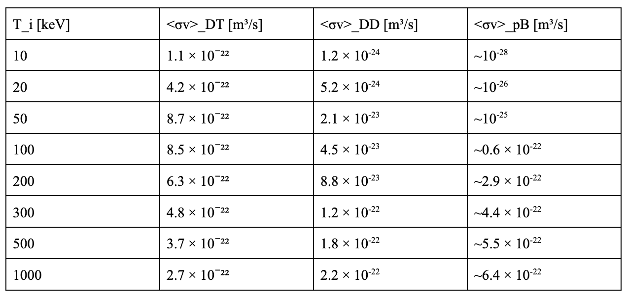
p–¹¹B reaction modeling for aneutronic fusion studies
The proton–boron reaction, p + ¹¹B → 3α + 8.68 MeV, is of interest as a potentially aneutronic fusion pathway. NSFsim development has included a preliminary physics study and the design of a modeling pipeline to integrate with the transport solver.
The aim is not to treat p–¹¹B as a simple extension of D–T or D–D modeling. The reaction has different temperature requirements, alpha-particle behavior, radiation constraints, and transport implications. A useful simulator must therefore represent the reaction in a way compatible with profile evolution, heating terms, and a self-consistent assessment of plasma performance.
We see this direction as relevant to both fundamental studies of p–B plasma physics and early-stage design analyses of next-generation aneutronic fusion concepts.
Scrape-off layer modeling
The scrape-off layer (SOL) is the region between the last closed flux surface and the divertor. It strongly influences heat and particle loads on plasma-facing components and therefore cannot be decoupled from practical tokamak design.
NSFsim is being extended with a hierarchy of SOL models that can be selected based on the required fidelity and computational cost.
Completed: 0D box model
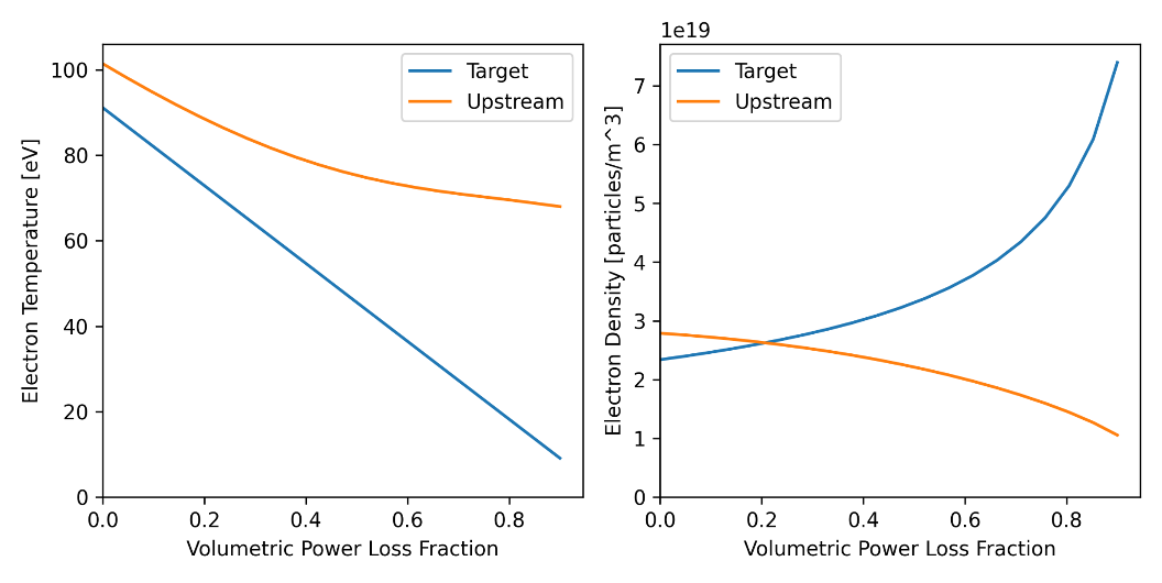
A fast analytical 0D box model has been implemented using a modified two-point formulation [3]. The model takes particle and heat fluxes from the core into the SOL as inputs and analytically estimates upstream and target parameters.
The implementation accounts for the actual geometry via the parallel connection length obtained from equilibrium. It also includes flux-expansion effects and uses the Goldston drift heuristic for the SOL width. Initial calculations for a CENTAUR-like negative-triangularity plasma, with 13.5 MW of SOL power and a heat-flux width of 1.3 mm, reproduce the expected dependence of the upstream and target electron temperatures and densities on the volumetric power-loss fraction.
Correction to the 1D box-model formulation
During testing of the analytical expressions in the reduced SOL model [3], we found that the expression under the square root can become negative near the target plate in certain parameter regimes. A correction has been introduced to handle these cases and extend the model's practical range.
In progress: onion model
The next step is the onion model, in which the SOL is decomposed into a set of one-dimensional flux tubes. Cross-field transport is provided by the NSFsim one-dimensional radial model. Each flux tube solves conservation equations for particles, parallel momentum, and electron and ion energy, with Bohm boundary conditions at the target and charge-state-resolved impurity support.
Because cross-field transport enters explicitly, this model provides a natural connection between the SOL and the core radial transport solver. The intended result is a scalable family of SOL models: from a millisecond-level engineering model to a higher-fidelity SOL solver, depending on the purpose of the calculation.
Summary
The recent NSFsim updates strengthen the simulator in three main ways.
First, the core forward and inverse workflows are becoming more physically transparent and easier to integrate with external physics modules. The transition to physical inverse-solver inputs and the improved inverse-to-forward initialization are particularly important for design studies.
Second, the simulator is becoming more useful for time-dependent and experiment-facing workflows. The scenario builder, equilibrium reconstruction module, diagnostic weighting, flexible coil-current management, and limited-data discharge initialization all support simulations that remain close to realistic tokamak operation.
Third, the roadmap extends NSFsim beyond core equilibrium and transport calculations. Three-dimensional structural currents, p–¹¹B reaction modeling, and a hierarchy of SOL models are being developed to address physics areas that are important for future device design and reactor-relevant studies.
The broader direction is clear: NSFsim is being developed as an integrated tokamak simulation environment rather than a single-purpose solver. The immediate priority is to add the physics most useful for current design, control, reconstruction, and benchmarking tasks.
We are open to collaborations and technical feedback from groups working on related modeling challenges.
References
[1] N. B. Marushchenko, Y. Turkin, H. Maaßberg, Ray-tracing code TRAVIS for ECR heating, EC current drive and ECE diagnostic, Computer Physics Communications 185 (2014) 165–176.
[2] J. Varje, K. Särkimäki, J. Kontula, P. Ollus, T. Kurki-Suonio, A. Snicker, E. Hirvijoki, S. Äkäslompolo, High-performance orbit-following code ASCOT5 for Monte Carlo simulations in fusion plasmas, arXiv:1908.02482.
[3] X. Zhang, F. M. Poli, E. D. Emdee, and M. Podestà, Reduced physics model of the tokamak Scrape-Off-Layer for pulse design, Nuclear Materials and Energy, vol. 34, 101354, 2023.
Next Step Fusion is a supply chain company supporting tokamak developers in the design, simulation, optimization, control, and operation of their devices through integrated modeling and AI/ML-enabled solutions.
We invite you to be part of this groundbreaking journey!
Follow our blog, subscribe to our LinkedIn for regular updates, watch our videos on YouTube, or reach out to us directly to discuss potential collaborations.